import matplotlib.pyplot as plt
import numpy as np
from scipy.optimize import fsolve

import matplotlib
import matplotlib.style as style
from matplotlib.pyplot import cm
from matplotlib.text import OffsetFrom
%matplotlib inline
style.use('bmh')
matplotlib.rcParams['axes.facecolor'] = 'ffffff'
import mplcursors
import labellines as ll

#Toggle printing for debugging
print_on = False
def print1(something='', somethingelse=''):
    if print_on == True: print(something, somethingelse)
import pygasflow
import pygasflow.isentropic as isen
some_mach_number = 3.5
isen.critical_area_ratio(some_mach_number)[0]  #checks out!, this gets A/A*  from M in isentropic tables
isen.m_from_critical_area_ratio(6.78962054, flag='sup')[0]
Good! "some_mach_number" was recovered, Python matches Anderson tables.
Increase the diameter step by step, the velocity change is modelled as instantaneous and shear acts along each section.
#LHS
def frict_lhs(delta_x, f):
    return ((4 * f) / (d)) * (delta_x)

#RHS (In brackets)
def frict_rhs(m):
    aa = 1 / (y * m**2)
    bb = (y + 1) / (2 * y)
    cc = np.log((m**2) / (1 + 0.5 * (y - 1) * m**2))
    return -aa - bb * cc

def frict_equals_zero(m2):
    return frict_rhs(m2) - frict_rhs(m1) - frict_lhs(delta_x, f)
Solving by hand: $M_2 = 2.8$
y = 1.4  #lambda
f = 0.005
m1 = 5
d = 0.2
delta_x = 2.04
print('Solving with python:')
print('M_2 = ', fsolve(func=frict_equals_zero, x0=2)[0])
The above function allows for calculating the mach number at state 2 without using the sonic intermediary
ndiameters  = 100
d_exit_array = np.linspace(0.2,1,ndiameters)

#Zoom in on answer
#d_exit_array = np.linspace(0.55,0.56,ndiameters)

Dexit_array_all = np.zeros(ndiameters)
mexit_array_all = np.zeros(ndiameters)


for j in range(ndiameters):
    ###########
    d_exit = d_exit_array[j]
    ###########
    m1=5
    f=0.005 #friction coef
    y=1.4  #lambda
    d_in = 0.2 #m

    #Break up the control volume into straight sections.
    nnodes=1000
    xf=2.04
    L = xf

    #The length of each straight section.
    delta_x=((xf)/(nnodes))  #m

    #The slope of Area vs. X , Diameter vs. X
    slopea = (np.pi * (d_exit**2 - d_in**2))   /   (4 * L)
    sloped = (d_exit - d_in) / L

    #These aren't used.
    p1=1
    t1=273

    d=d_in
    area_in=np.pi*((d_in**(2))/(4))

    x1=0
    y=1.4

    #set innital conditions
    area1=area_in
    d=d_in

    #X values and Mach numbers along the length of the duct.
    x2_array = np.zeros(nnodes)
    m2_array = np.zeros(nnodes)


    for i in range(nnodes):

        x2 =x1+delta_x
        print1( "x2=",x2)
        print1( "m1=",m1)

        #Apply friction to the straight section, Solve for M_2.
        starting_guess = m1-1
        m2_temp = fsolve(frict_equals_zero, starting_guess)
        m2 = m2_temp[0]

        m1=m2
        print1( "m1'=",m1)

        #Applying the increase in area, solve for new M_3.
        #New diameter after the diameter increase.
        d2 = d + sloped*delta_x

        #New area after the diameter increase.
        area2= 0.25 * np.pi * d2**2

        #Area ratio is used in the tables.
        ratioa_i=((area2)/(area1))

        #Get a / a*
        a1prime_astr=isen.critical_area_ratio(m1)[0]

        print1( "ratioa_i=",ratioa_i)

        #Calculate A2/A*
        a2_astr=a1prime_astr*ratioa_i

        #Get M_3 from a "reverse lookup" in the tables, M2 as a function of A2/A*.
        m2=isen.m_from_critical_area_ratio(a2_astr,flag='sup')[0]
        print1("~m2=",m2)

        #Get ready for next loop.
        x1=x2
        m1=m2
        area1=area2
        d=(((4*area2)/(np.pi)))**(0.5)
        print1("---")

        #dump values to array
        x2_array[i] = x2
        m2_array[i] = m2

    print1( "++++++++++++++++++")
    print1("d_exit=",d)
    print1("A_exit=",area1)

    Dexit_array_all[j] = d_exit
    mexit_array_all[j] = m2

    #print('D_exit=',d_exit)
    print1('M_exit = ',m2)
#Interpolate M_exit -vs- Diameter_exit for M_exit=5, this will be the solution!
D_exit_ANSWER = np.interp(5,mexit_array_all,Dexit_array_all)

#Everything past here is just plotting.
fig1,ax1 = plt.subplots(figsize=(8,6),dpi=100)

plt.vlines(D_exit_ANSWER,mexit_array_all[0],5,linestyles='--',alpha=0.2)
plt.hlines(5,0.2,D_exit_ANSWER,linestyles='--',alpha=0.2)

plt.plot(Dexit_array_all,mexit_array_all,label='$M_{exit}$')
plt.scatter(D_exit_ANSWER,5,s=100,c='r',label='For constant Mach flow')

plt.title('Variable Area Duct Flow with Friction')
plt.ylabel('Mach Number at Exit')
plt.xlabel('Diameter at Exit')

plt.grid(True)
mplcursors.cursor(hover=True)

plt.legend()
plt.show()

def D2Alpha(d_exit):
    return np.arctan((d_exit - d_in) / (2 * L)) * (180 / np.pi)

print('RESULT:')
print('D_exit =',D_exit_ANSWER, 'meters')
print('α =',D2Alpha(D_exit_ANSWER),'°')

ndiameters  = 100


#Zoom in on answer  0.5569
d_exit_array = np.linspace(0.5565,0.5572,ndiameters)

Dexit_array_all = np.zeros(ndiameters)
mexit_array_all = np.zeros(ndiameters)

for j in range(ndiameters):
    ###########
    d_exit = d_exit_array[j]
    ###########
    m1=5
    f=0.005 #friction coef
    y=1.4  #lambda
    d_in = 0.2 #m

    #Break up the control volume into straight sections.
    nnodes=3000
    xf=2.04
    L = xf

    #The length of each straight section.
    delta_x=((xf)/(nnodes))  #m

    #The slope of Area vs. X , Diameter vs. X
    slopea = (np.pi * (d_exit**2 - d_in**2))   /   (4 * L)
    sloped = (d_exit - d_in) / L

    #These aren't used.
    p1=1
    t1=273

    d=d_in
    area_in=np.pi*((d_in**(2))/(4))

    x1=0
    y=1.4

    #set innital conditions
    area1=area_in
    d=d_in

    #X values and Mach numbers along the length of the duct.
    x2_array = np.zeros(nnodes)
    m2_array = np.zeros(nnodes)

    for i in range(nnodes):

        x2 =x1+delta_x
        print1( "x2=",x2)
        print1( "m1=",m1)

        #Apply friction to the straight section, Solve for M_2.
        starting_guess = m1-1
        m2_temp = fsolve(frict_equals_zero, starting_guess)
        m2 = m2_temp[0]

        m1=m2
        print1( "m1'=",m1)

        #Applying the increase in area, solve for new M_3.
        #New diameter after the diameter increase.
        d2 = d + sloped*delta_x

        #New area after the diameter increase.
        area2= 0.25 * np.pi * d2**2

        #Area ratio is used in the tables.
        ratioa_i=((area2)/(area1))

        #Get a / a*
        a1prime_astr=isen.critical_area_ratio(m1)[0]

        print1( "ratioa_i=",ratioa_i)

        #Calculate A2/A*
        a2_astr=a1prime_astr*ratioa_i

        #Get M_3 from a "reverse lookup" in the tables, M2 as a function of A2/A*.
        m2=isen.m_from_critical_area_ratio(a2_astr,flag='sup')[0]
        print1("~m2=",m2)

        #Get ready for next loop.
        x1=x2
        m1=m2
        area1=area2
        d=(((4*area2)/(np.pi)))**(0.5)
        print1("---")

        #dump values to array
        x2_array[i] = x2
        m2_array[i] = m2

    print1( "++++++++++++++++++")
    print1("d_exit=",d)
    print1("A_exit=",area1)

    Dexit_array_all[j] = d_exit
    mexit_array_all[j] = m2

    print1('M_exit = ',m2)
#Interpolate M_exit -vs- Diameter_exit for M_exit=5, this will be the solution!
D_exit_ANSWER = np.interp(5,mexit_array_all,Dexit_array_all)

#Everything past here is just plotting.
fig1,ax1 =  plt.subplots(figsize=(8,6),dpi=100)

plt.vlines(D_exit_ANSWER,mexit_array_all[0],5,linestyles='--',alpha=0.2)
plt.hlines(5,Dexit_array_all[0],D_exit_ANSWER,linestyles='--',alpha=0.2)

plt.plot(Dexit_array_all,mexit_array_all,label='$M_{exit}$')
plt.scatter(D_exit_ANSWER,5,s=100,c='r',label='For constant Mach flow')

plt.title('Variable Area Duct Flow with Friction')
plt.ylabel('Mach Number at Exit')
plt.xlabel('Diameter at Exit')

plt.grid(True)
mplcursors.cursor(hover=True)

plt.legend()
plt.show()

def D2Alpha(d_exit):
    return np.arctan((d_exit - d_in) / (2 * L)) * (180 / np.pi)

print('RESULT:')
print('D_exit =',D_exit_ANSWER, 'meters')
print('α =',D2Alpha(D_exit_ANSWER),'°')

also increase resolution
d_in = 0.2 #m
d_exit = D_exit_ANSWER #m

nnodes=100000
x1=0
xf=2.04
L = xf

delta_x=((xf)/(nnodes))
m1=5

y=1.4  #lambda
f=0.005

slopea = (np.pi * (d_exit**2 - d_in**2))   /   (4 * L)
sloped = (d_exit - d_in) / L

p1=1
t1=273

area_in=np.pi*((d_in**(2))/(4))

#set innital conditions
area1=area_in
d=d_in

x2_array = np.zeros(nnodes)
A2_array = np.zeros(nnodes)

m2_array = np.zeros(nnodes)
D_array = np.zeros(nnodes)


for i in range(nnodes):

    x2 =x1+delta_x
    print1( "x2=",x2)
    print1( "m1=",m1)

    starting_guess = m1-1
    m2_temp = fsolve(frict_equals_zero, starting_guess)
    m2 = m2_temp[0]

    m1=m2
    print1( "m1'=",m1)

    d2 = d + sloped*delta_x
    area2= 0.25 * np.pi * d2**2

    ratioa_i=((area2)/(area1))
    a1prime_astr=isen.critical_area_ratio(m1)[0]

    print1( "ratioa_i=",ratioa_i)

    a2_astr=a1prime_astr*ratioa_i
    m2=isen.m_from_critical_area_ratio(a2_astr,flag='sup')[0]
    print1("~m2=",m2)

    x1=x2
    m1=m2
    area1=area2
    d=(((4*area2)/(np.pi)))**(0.5)
    print1("---")

    #dump values to array
    x2_array[i] = x2
    m2_array[i] = m2
    D_array[i] = d
    A2_array[i] = area2


r_array = 0.5 * D_array
print1( "++++++++++++++++++")
print1("d_exit=",d)
print1("A_exit=",area1)

print('D_exit=',d_exit)
print('M_2 FINAL = ',m2)

print('')
#PLOTING
fig1,ax1 =  plt.subplots(figsize=(8,6),dpi=100)
plt.plot(x2_array,m2_array,label='M(x)')

plt.title('Mach Number along x Axis \nVariable Area Duct Flow with Friction ')
plt.ylabel('M')
plt.xlabel('x')
plt.legend()
#mplcursors.cursor(hover=True)
plt.grid(True)

#plt.ylim((4.999,5.001))
plt.show()

print('M_inlet = ', 5)
print('M_exit = ',m2_array[-1])

Above shows the mach distribution of the solution (constant mach flow)
plt.figure(figsize=(10,5))

for i in range(20):
    plt.plot([x2_array[i],x2_array[i+1]],[r_array[i],r_array[i]],c='r')
    plt.plot([x2_array[i+1],x2_array[i+1]],[r_array[i],r_array[i+1]],c='r')


plt.xlim((x2_array[1],x2_array[5]))
plt.ylim((0.1,0.1+1e-5))
plt.title('Duct is broken up into small straight sections')
plt.ylabel('Radius  (meters)')
plt.ticklabel_format(style='sci', axis='x', scilimits=(0,0))
plt.show()


plt.figure(figsize=(10,5))
for i in range(20):
    plt.plot([x2_array[i],x2_array[i+1]],[-r_array[i],-r_array[i]],c='r')
    plt.plot([x2_array[i+1],x2_array[i+1]],[-r_array[i],-r_array[i+1]],c='r')

plt.xlim((x2_array[1],x2_array[5]))
plt.ylim((-0.1-1e-5,-0.1))
plt.ylabel('Radius  (meters)')
plt.xlabel('Distance along duct (meters)')
plt.ticklabel_format(style='sci', axis='x', scilimits=(0,0))
plt.show()


def nozz_plot_mach(title_below=''):

    fig3, ax3 = plt.subplots(figsize=(13,8),dpi=300)
    plt.plot(x2_array,r_array,c='k')
    plt.plot(x2_array,-r_array,c='k')
    plt.title('Diffuser Geometry, Mach Number \n'+title_below)
    plt.axis('equal')

    n_fill_lines = 110
    noz_mask = np.linspace(-1.5,1.5,n_fill_lines)
    for i in range(n_fill_lines):
        plt.scatter(x2_array,x2_array*0 + noz_mask[i],label='M(x)'
                    ,c=m2_array,cmap='plasma',lw=1,marker='s')
    #FILL ABOVE NOZZLE
    ax3.fill_between(x2_array, r_array, 3+r_array,facecolor='white',cmap='plasma')

    #FILL BELOW NOZZLE
    ax3.fill_between(x2_array, -r_array, -(3+r_array),facecolor='white',cmap='plasma')

    #FILL ON LHS OF NOZZLE
    ax3.fill_between([-2,0.01], [-2,-2], [2,2],facecolor='white',cmap='plasma')

    #FILL ON RHS OF NOZZLE
    ax3.fill_between([L,L+1], [-2,-2], [2,2],facecolor='white',cmap='plasma')

    plt.xlim(-0.1,2.2)
    plt.ylim((-r_array[-1] ,r_array[-1]))
    plt.ylabel('r (meters)')
    plt.xlabel('x (meters)')

    plt.colorbar()
    plt.show()
fig4, ax4 = plt.subplots(figsize=(13, 8), dpi=300)

#f_array = np.arange(0,0.021,0.0025)
f_array = [
    0, 0.001, 0.002, 0.003, 0.004, 0.005, 0.007, 0.01, 0.015, 0.025, 0.0365
]

color = cm.rainbow(np.linspace(0, 1, np.size(f_array)))
d_exit = D_exit_ANSWER

for j in range(np.size(f_array)):
    f = f_array[j]

    d_in = 0.2  #m
    area_in = np.pi * ((d_in**(2)) / (4))

    nnodes = 1000
    x0 = 0
    x1 = 0
    xf = 2.04
    L = xf

    delta_x = ((xf) / (nnodes))
    m1 = 5

    y = 1.4  #lambda

    slopea = (np.pi * (d_exit**2 - d_in**2)) / (4 * L)

    sloped = (d_exit - d_in) / L

    p1 = 1
    t1 = 273

    #set innital conditions
    area1 = area_in
    d = d_in

    x2_array = np.zeros(nnodes)
    m2_array = np.zeros(nnodes)
    D_array = np.zeros(nnodes)

    for i in range(nnodes):

        x2 = x1 + delta_x
        print1("x2=", x2)
        print1("m1=", m1)

        starting_guess = m1 - 1
        m2_temp = fsolve(frict_equals_zero, starting_guess)
        m2 = m2_temp[0]

        m1 = m2
        print1("m1'=", m1)

        d2 = d + sloped * delta_x
        area2 = 0.25 * np.pi * d2**2

        ratioa_i = ((area2) / (area1))
        a1prime_astr = isen.critical_area_ratio(m1)[0]

        print1("ratioa_i=", ratioa_i)

        a2_astr = a1prime_astr * ratioa_i
        m2 = isen.m_from_critical_area_ratio(a2_astr, flag='sup')[0]
        print1("~m2=", m2)

        x1 = x2
        m1 = m2
        area1 = area2
        d = (((4 * area2) / (np.pi)))**(0.5)
        print1("---")

        #dump values to array
        x2_array[i] = x2
        m2_array[i] = m2
        D_array[i] = d

    print1("++++++++++++++++++")
    print1("d_exit=", d)
    print1("A_exit=", area1)

    print1('D_exit=', d_exit)
    print1('M_2 FINAL = ', m2)

    plt.plot(x2_array,
             m2_array,
             c=color[j],
             label=r'$f =$' + '{:0.3f}'.format(f))

plt.title(
    ' Mach Number along x Axis \n Variable Area Duct Flow with Friction \n' +
    r'$\alpha = 5 \degree$')
plt.ylabel('M')
plt.xlabel('x')

box = ax4.get_position()
ax4.set_position([box.x0, box.y0, box.width * 0.8, box.height])

plt.legend(loc='upper right',
           ncol=1,
           bbox_to_anchor=(1.2, 1),
           borderaxespad=0,
           frameon=True)

plt.grid(True)
ll.labelLines(plt.gca().get_lines(),
              zorder=2.5,
              align=False,
              fontsize=7,
              ha='center',
              color='k',
              xvals=(1.8, 1.8))
#mplcursors.cursor(hover=True)
plt.show()
r_array = 0.5 * D_array

nozz_plot_mach(title_below=r'$\alpha = 5 \degree , f = 0.036$')

Above shows the case where friction 'wins' and the flow slows down.
fig5, ax5 = plt.subplots(figsize=(13, 8), dpi=300)

#Based on d_exit
d_exit_array = np.array([0.2, 0.3, 0.4, 0.5, D_exit_ANSWER, 0.7, 0.8, 0.9, 1])
alpha_array = np.arctan((d_exit_array - d_in) / (2 * L)) * (180 / np.pi)

#Based on alpha
alpha_array = np.array([0, 1, 2, 3, 4, 5, 6, 7, 8, 9, 10])
d_exit_array = np.tan(alpha_array * (np.pi / 180)) * L * 2 + d_in

color = cm.rainbow(np.linspace(0, 1, np.size(d_exit_array)))
for j in range(np.size(d_exit_array)):

    ################
    #VARY THE EXIT DIAMETER
    d_exit = d_exit_array[j]
    ###############
    d_in = 0.2  #m
    nnodes = 1000
    x1 = 0
    xf = 2.04
    L = xf
    delta_x = ((xf) / (nnodes))
    m1 = 5
    y = 1.4  #lambda
    f = 0.005
    slopea = (np.pi * (d_exit**2 - d_in**2)) / (4 * L)
    sloped = (d_exit - d_in) / L

    p1 = 1
    t1 = 273
    area_in = np.pi * ((d_in**(2)) / (4))

    #set innital conditions
    area1 = area_in
    d = d_in

    #Blank
    x2_array = np.zeros(nnodes)
    m2_array = np.zeros(nnodes)
    D_array = np.zeros(nnodes)

    for i in range(nnodes):

        x2 = x1 + delta_x
        print1("x2=", x2)
        print1("m1=", m1)

        starting_guess = m1 - 1
        m2_temp = fsolve(frict_equals_zero, starting_guess)
        m2 = m2_temp[0]

        m1 = m2
        print1("m1'=", m1)

        d2 = d + sloped * delta_x
        area2 = 0.25 * np.pi * d2**2

        ratioa_i = ((area2) / (area1))
        a1prime_astr = isen.critical_area_ratio(m1)[0]

        print1("ratioa_i=", ratioa_i)

        a2_astr = a1prime_astr * ratioa_i
        m2 = isen.m_from_critical_area_ratio(a2_astr, flag='sup')[0]
        print1("~m2=", m2)

        #FOR THE NEXT LOOP
        x1 = x2
        m1 = m2
        area1 = area2
        d = (((4 * area2) / (np.pi)))**(0.5)
        print1("---")

        #dump values to array
        x2_array[i] = x2
        m2_array[i] = m2
        D_array[i] = d

    print1("++++++++++++++++++")
    print1("d_exit=", d)
    print1("A_exit=", area1)

    print1('D_exit=', d_exit)
    print1('M_2 FINAL = ', m2)
    print1('')

    #nozz_plot_mach(title_below=r'$\alpha = $'+'{}°'.format(alpha_array[j]))

    #PLOTING
    #plt.plot(x2_array,m2_array,c=color[j],label=r'$d_{exit} = $'+'{:0.3f} m'.format(d))
    plt.plot(x2_array,
             m2_array,
             c=color[j],
             label=r'$\alpha = $' + '{:0.2f}°'.format(alpha_array[j]))

r_array = 0.5 * D_array

plt.title(
    ' Mach Number along x Axis \n Variable Area Duct Flow with Friction \n' +
    r'$f = 0.005$')
plt.ylabel('M')
plt.xlabel('x (meters)')
plt.legend()

box = ax5.get_position()
ax5.set_position([box.x0, box.y0, box.width * 0.8, box.height])

plt.legend(loc='upper right',
           ncol=1,
           bbox_to_anchor=(1.2, 1),
           borderaxespad=0,
           frameon=True)

mplcursors.cursor(hover=False)
plt.grid(True)
#ll.labelLines(plt.gca().get_lines(),zorder=2.5,align=False,fontsize=8,ha='center',color='k',xvals=(1,1))
ll.labelLines(plt.gca().get_lines(),
              zorder=2.5,
              align=False,
              fontsize=7,
              ha='center',
              color='k',
              xvals=(1.8, 1.8))  #,

plt.show()

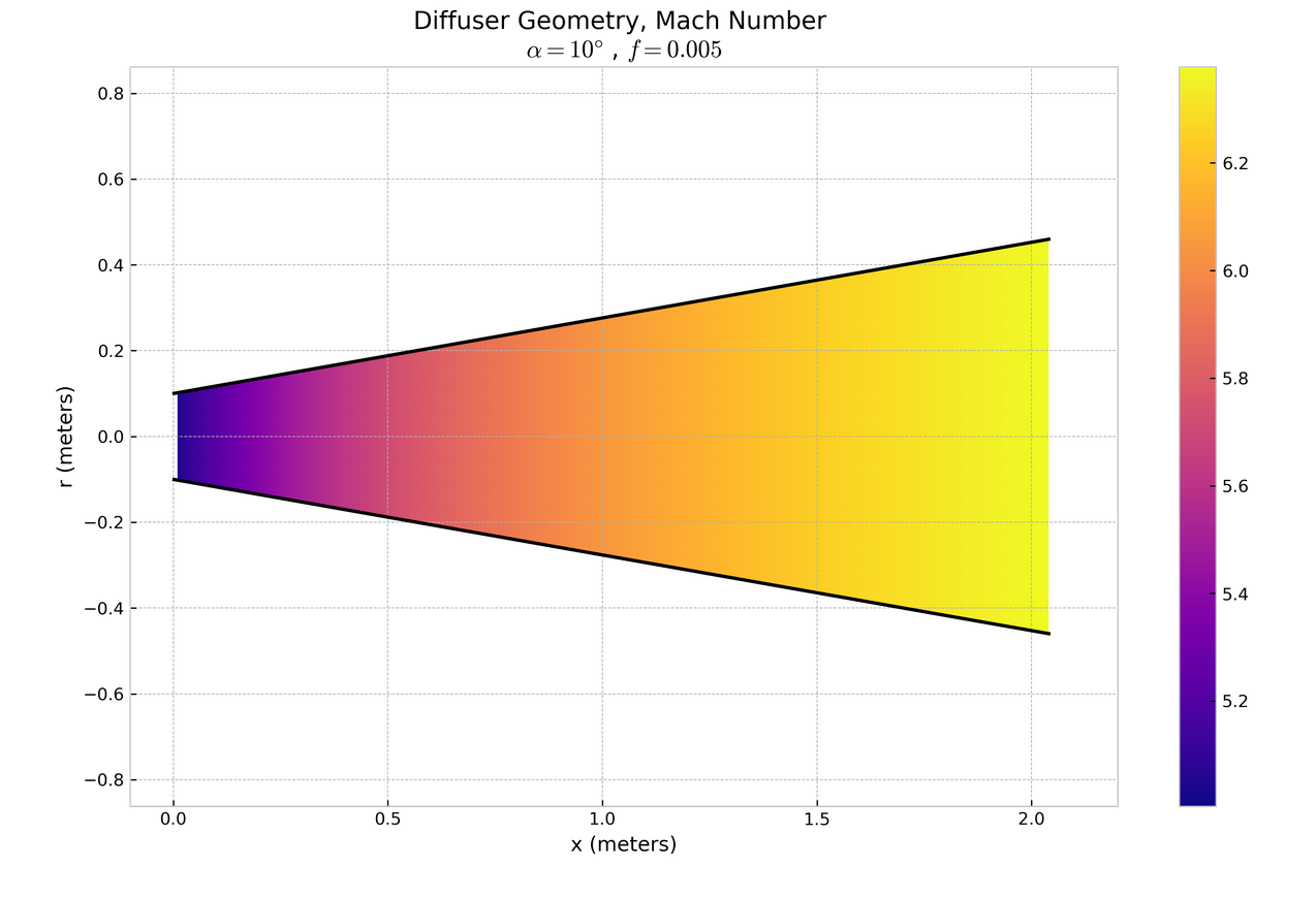
nozz_plot_mach(title_below=r'$\alpha = 10 \degree$ , $f=0.005$')

Above shows the case where area-change 'wins' and the flow speed increases.